VLOOKUP – How to get from zero to hero – Part 1

Some time ago I was asked to explain how the Excel Vlookup formula works. I have been using this formula for many years, it’s easy and fast to implement, and with a few tweaks, it can be expanded.

The formula

VLOOKUP is the acronym for Vertical Lookup. What the formula does, is to look for a value in an area of your spreadsheet and if that value is found it returns the correspondent value that sits in a column on the right.

VLOOKUP needs three parameters and an optional one (in square brackets below)

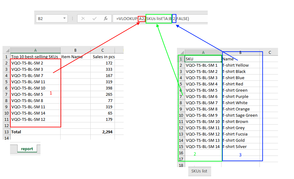
=VLOOKUP(lookup_value,table_array,col_index_num,[range_lookup])

If you need a quick way to remember the parameters then this is what you have to remember:

=VLOOKUP(what, where, n# of columns on the right, false)

Note, I have always used “false” in the last parameter because I always want the exact match of what I am looking for. If you want the closest match then replace “false” with “true”.

The basic usage

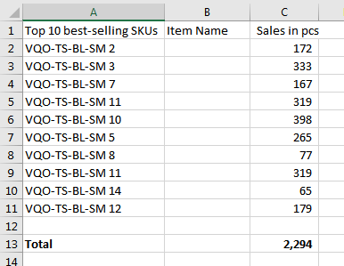
Let’s say you have two Excel sheets, “report” with the top 10 best-selling SKUs with the relevant units sold, and “SKUs list” with a collection of SKUs with the appropriate name beside. You want to show the item name for each of the top 10 best-selling SKUs in the first sheet to make it more readable.

The three elements are

1. The value to be looked for is each SKU in “report”.
2. The area to look into is the collection of SKUs “in the second sheet.”SKUs list”.
3. The value to be returned can be found in the second column of “SKUs list”

If you want to download the example above, please click here