VLOOKUP INDEX/MATCH- How to get from zero to hero – Part 3

The method in part 2 works fine and this is the one I use most of the time, the only drawback is you need the helping column. Besides, VLOOKUP returns the values you need on the right of the search column, which is a limitation. There are ways to get around both issues but these are either overly complicated or require more columns. A better and faster way to solve all these issues is to combine INDEX and MATCH formulas.

Let’s break down the task into smaller bits.

The INDEX formula

This formula returns a value from a selected range by its position, hence its name.

This is the syntax:

INDEX(array, row, [column])

• array is the range we want to consider
• row, and column if necessary, identify the position of the value we seek.

Here is the basic use

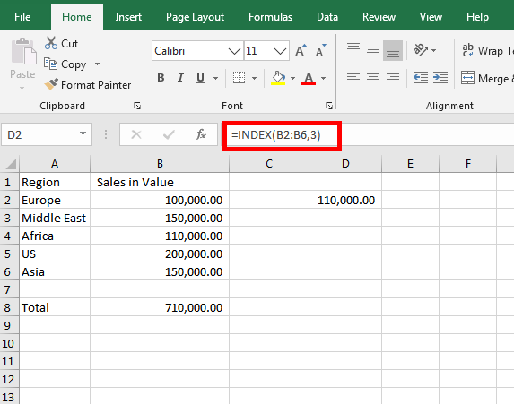
In this case, INDEX considers the array B2:B6 and returns the value in the row 3. We don’t need the parameter “column” in this formula because the array has one column only

The example below refers to an array of multiple columns instead, this will need the parameter “column”. This reminds me of the Sea Battle paper game.

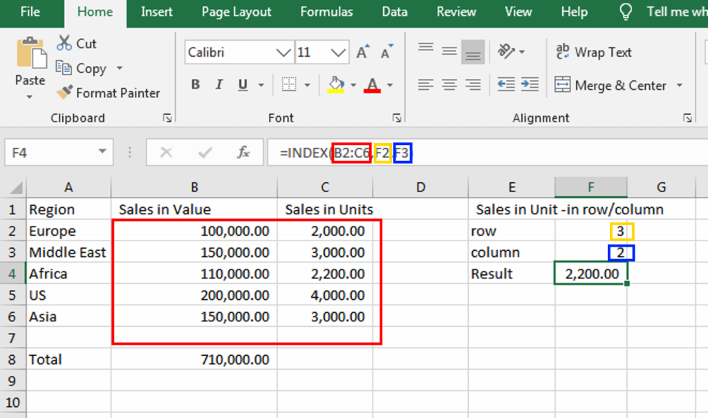
Here, INDEX considers the array B2:C6 and returns the value in row 3 (taken from cell F2) and column 2 (taken from cell F3).

Now we have found a way to locate a specific value in a range, but how can we automatically find the right row and column value? This is something that MATCH can help with!

The MATCH formula

This formula is designed to find the position of a value in a range. Here is the syntax

MATCH(lookup_value, lookup_array, [match_type])

• lookup_value is the value we are looking for
• lookup_array is the range we are looking at for the lookup_value
• match_type can have two values:
  • If it is 0 then MATCH looks for a perfect match
  • If it is 1 then the formula will find the closest match. I always use 0

here there are a couple of examples

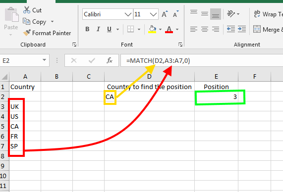
In the example above, MATCH finds the value in D2 in the range A3:A7 and returns it in cell E2.

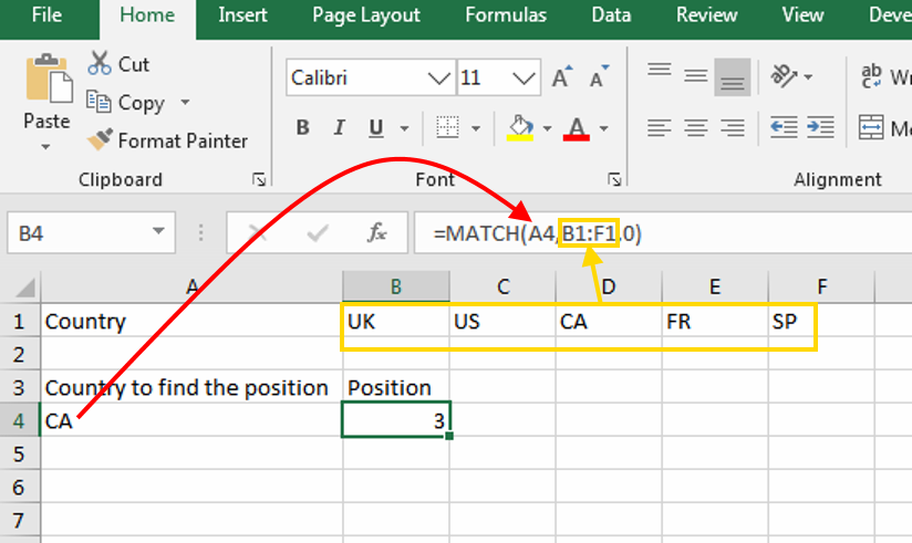
One important feature of MATCH is the formula works even when the range is distributed horizontally.

Combining the two formulas

At this stage, we have learned how to find the position of a value in a range and how to find where this value is positioned in a range. It is now the moment to combine the two.

Let’s say you have this table with unit sales figures, broken down by country, month, and salespeople names.

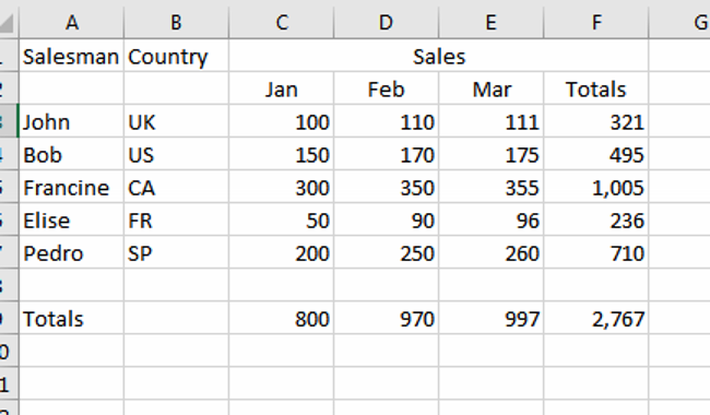
Your task is to find how many units were sold in a specific country and by which salesperson.

We start by finding which line the country we are looking for is and use MATCH for this.

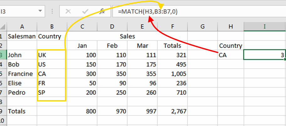
The value “CA” we are looking for is in cell H3 and the range we are looking into is B3:B7. MATCH returns 3 because the value “CA” is in the third line of the range. The result is in cell I3

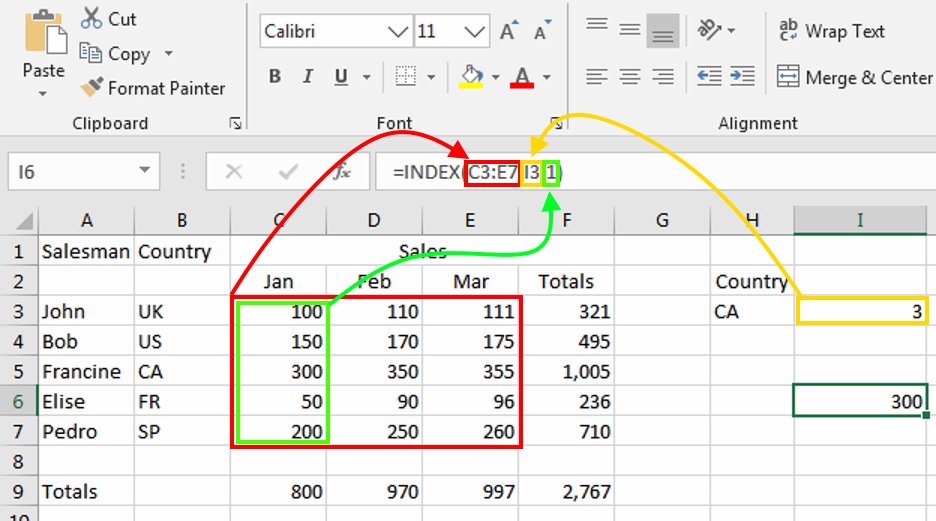
Next, is the INDEX formula

The first parameter C3:E7 is the range where the data we want to find resides (the red area below), the second, I3 (the yellow rectangle), is the range line number we have seen in the above paragraph and the third, “1” (the green rectangle), is the range column number to refer to (we want the value from the column “Jan”). In practice, we want the value in line 3, column 1 of the range C3:E7. The result is 300, in cell I6, as this is the sales in Canada for January.

dated.

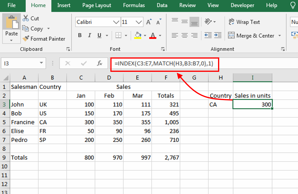
The next step is to combine the two formulas in one cell

As you may have noticed this is just a more complicated way to achieve what can be achieved with VLOOKUP. Here below is a picture that shows a comparison between INDEX/MATCH and VLOOKUP.

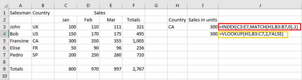
In column “J” you will see both formulas, in column “I” the relevant results. So, what is the point of making our life harder?

INDEX/MATCH search both ways

The answer is, INDEX/MATCH can return values on the right AND the left of the search column, VLOOKUP instead of only on the right! In the next example, I will show.

In the final example, we find the salesperson in addition to the sales figures.

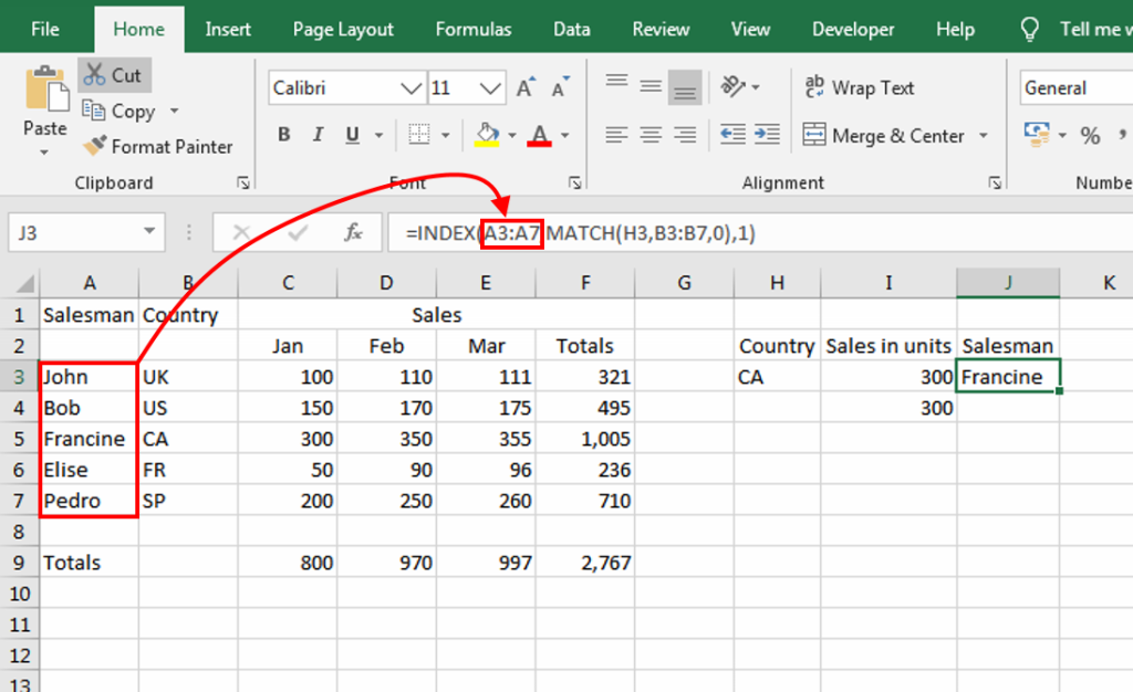
The column where we want the result from, (the salesman column “A” in red), is at the left of the search column (the country in column “B”). Being on the left of the main search column “B”, VLOOKUP cannot retrieve it.

If you download the spreadsheet file here you can play around with the example above.