VLOOKUP – How to get from zero to hero – Part 2

Sometimes you need to go beyond the basics of the VLOOKUP formula, a typical example is to locate data based on multiple columns. The trick is to concatenate the data.

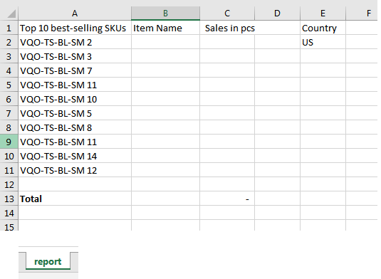
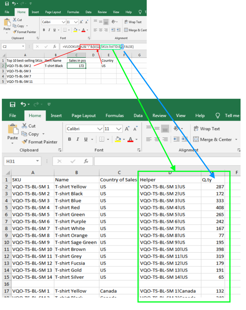
In this example you have some data, similar to the previous example but this time you have to locate the best-selling items for a specific country.

These are the two sheets:

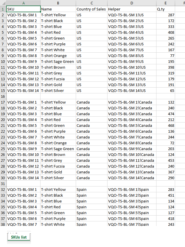
As VLOOKUP can search a value in one column only, you need to create a helper column in the tab “SKUs list” that combines the SKU and the Country for each item (I have also added a “!” for clarity but this may not be necessary in real applications).

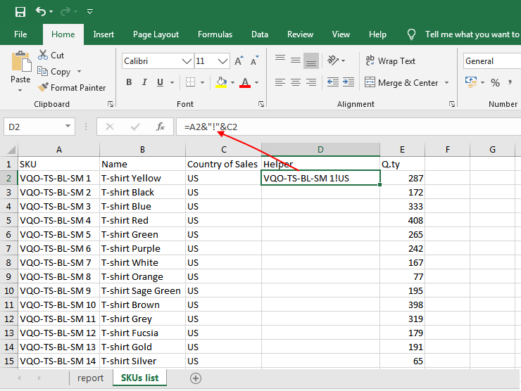
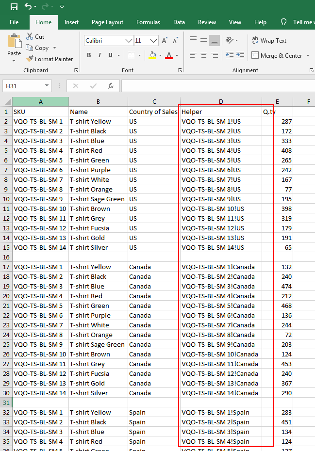
copy/paste the formula down in column “D” now. This will be the value identifying SKU and Country for each item.

=VLOOKUP(A2&"!"&$E$2,'SKUs list'!D:E,2,FALSE)

• A2&"!"&$E$2 combines the SKU and the country in cell E2, note the “$” to keep this cell reference fixed as the Country will not change when it comes to copying the formula down.
• 'SKUs list'!D:E selects the area where A2&"!"&$E$2 must be looked for.
• 2, this is to instruct the formula to return the data in the second column if A2&"!"&$E$2 is found in 'SKUs list'!D:E.
• False is to instruct the formula that we are interested only in perfect matches of A2&"!"&$E$2.

If you want to download this exercise, click here.